Introduction 

Excel is a powerful tool with many functions for manipulating and formatting data. This class will explore about 20 formulas, but these are just the tip of the iceberg. Excel has roughly 350 built-in formulas, depending on the version you use, but being able to use just a handful of them proficiently will go a long way in helping you get what you need from your data, and getting the data properly formatted to import into PowerSchool.

In this course, you’ll learn how to:

• Use formulas to properly format data for importing into PowerSchool
• Use formulas to add to, extract from, combine, and alter different types of data

Getting Started In Excel

Before diving into the functions that are available in Excel, first become familiar with some terms that will be used throughout this course. Then learn how to open files in the format that PowerSchool exports: delimited text.

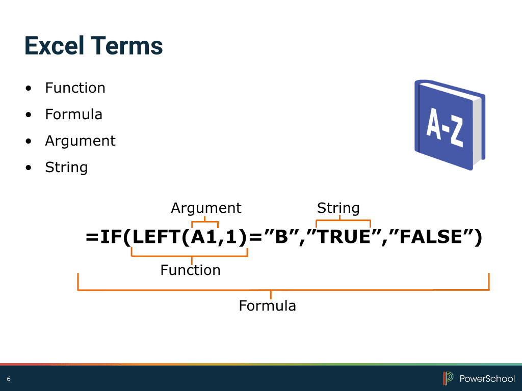
• Function – a built-in rule that tells Excel what to do with the arguments contained within it
• Formula – usually made up of one or more functions and dictates the value displayed in a cell
• Arguments – the variable parts of a function, separated by commas, that determine the result
• String – a collection of characters that Excel considers to be text; usually a string contains at least one letter
  
  Refer to the figure on Excel terms to see a sample formula with labels for each of its parts.

Interaction 1 - Slides

Using Built-In Tools

Excel has several built-in tools that make some basic formatting and data manipulation tasks quick and easy. These aren’t formulas, but rather selectable actions that you can perform on a cell or group of cells.

“Find and Replace”

The first handy tool is Excel’s “Find and Replace” feature. This works similarly to Word’s “Find and Replace” feature, and is a quick way to replace a fixed string of text within another, larger string.

Interaction 2 – Slides

Activity 1 – Using The “Find and Replace” Feature

Phone numbers in your data file aren’t all in the same format. Use “Find and Replace” to remove any characters beyond the numbers. Then change the cell format so the phone numbers all appear in the format (XXX) XXX-XXXX.

1. Open the ExcelAdapt_Activities.xlsx file
    
2. Verify you’re on the Student Info worksheet
    
3. Select the data in the Student Phone column by clicking cell C2, then pressing Command + Shift + the down arrow. Excel 2013 users, click cell C2, and then press Ctrl + Shift + the down arrow
    
4. Press Ctrl + H to open the Replace window
   Selecting the column data limits the changes you make using the “Find and Replace” function to the selected range of cells.
    
5. In the “Find what” field, enter ( and leave the “Replace with” field blank
   Leaving the second field blank will cause the search term to be deleted from the selected range of cells.
    
6. Click Replace All
   Notice that all open parentheses have been removed.
    
7. Click OK to confirm the number of changes
    
8. With the column still selected, repeat the find and replace process with the following characters separately:
   )
   -
   A blank space (type a single space in the “Find what” field; all spaces will be removed from the selected cells) When you’re done, you should have phone numbers with no characters between the digits.
    
9. Close the Replace window
    
10. With the data in the Student Phone column still selected, right-click the selected cells, and choose Format Cells from the menu
     
11. On the Number tab, select the Special category and choose Phone Number
     
12. Click OK

“Text To Columns”

There may be times when you want to split one column of cells, each containing several pieces of data, into multiple columns. Perhaps a column has both first and last names and you want to separate them, or maybe a delimited text file was imported, but not split by the delimiters so multiple columns of data got inserted into one.

As long as there’s a common delimiter in the cells, use “Text to Columns” to separate the data.

Interaction 3 – Slides

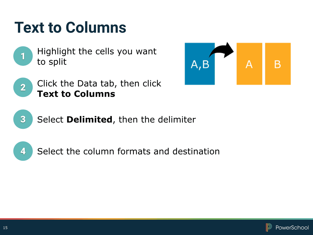
Review how to split a column of data into multiple columns. Click to view slide(s).

Activity 2 – Using the ”Text To Columns” Feature

Divide a column of teacher names into separate columns for their first, middle, and last names.

1. In the ExcelAdapt_Activities.xlsx file, select the Teacher Info worksheet
    
2. Select the data in the Full Teacher Names column, excluding the column heading
    
3. Click the Data tab in the ribbon, and then click Text to Columns
    
4. Verify that Delimited is selected as the file type and click Next
    
5. Select Comma and Space as the delimiters, clear the Tab check box, and then click Next
   When any of the selected delimiters appears, a break in the data occurs. Since there’s both a comma and a space between the last and first names, but only a space between first names and middle initials, be sure to keep Treat consecutive delimiters as one selected. This way last names, first names, and middle initials will all be broken out into separate columns.
    
6. Enter C2 as the destination; this is the cell where the data set will start
   Take a look at the “Data preview” area. Here you can get an idea of where your data will split and what it will look like.
    
7. Click Finish
    
8. Scroll down the list of names and manually fix any entries that split when they shouldn’t have
   Since a space is a delimiter, any first names with a space get split into separate columns.

Conditional Formatting

Use the conditional formatting tool to apply your chosen formatting to cells in a range that meet your selected condition(s). One useful way to use conditional formatting is to identify and highlight duplicate values.

Activity 3 – Using The Conditional Formatting Feature

Use conditional formatting to find and remove duplicate records on the State Exam worksheet.

1. Select the State Exam worksheet
    
2. Select the data in the Student ID column, excluding the column heading
    
3. On the Home tab of the Ribbon, click Conditional Formatting, and then choose New Rule
    
4. Mac users, in the window that appears, select Classic from the Style menu (Excel 2013 users skip this step)
    
5. Then select Format only unique or duplicate values
    
6. Ensure duplicate is selected in the next menu, and choose a formatting option for the cells containing duplicates. Notice that the cells with duplicates now have the formatting you selected.
    
7. Click OK
    
8. Filter the worksheet to show only the records that are duplicates
   1.With any single cell selected, click the Data tab in the Ribbon, and click the Filter button
   2. Open the Filter menu for the Student Number column
   3. In the Filter window, open the By Color menu and select the color you chose to apply to the duplicate values
   4. Close the Filter window – Only the duplicate records appear now
    
9. Sort the worksheet by Student Number so the duplicates appear next to each other
   1. With a single cell in the Student Number column selected, click the Data tab in the Ribbon
   2. Click the Sort Ascending button
    
10. Delete one of each of the duplicate records
     
11. Clear and remove the filter by clicking the Filter button in the Ribbon

Using Text Functions

Some functions in Excel typically apply to cells containing text strings, while others typically apply to cells containing numerical values. In most cases, Excel considers a cell’s value a text string if it contains at least one letter. Examples include names, addresses, and usernames. While you can’t perform mathematical operations on text strings, there are many ways you can reformat, add to, or extract information from them.

After entering a formula into a cell, apply it to the rest of a column using Autofill. Autofill enters the formula into the selected cells, and updates any cell references. To use Autofill, select the cell with the formula to be copied. Then move your cursor to the lower-right corner of the cell so it turns into a black + sign. Click and drag down the column, or double-click to autofill the formula down to the last populated row.

Also, there may be times when you want to include a string of text as part of a formula. Put the text in quotes to refer to the text as you’ve typed it, rather than having it be part of a cell reference or other operation. This is useful when you want to insert specific text into the same place in multiple cells, or you want a string of text considered as an argument in a formula.

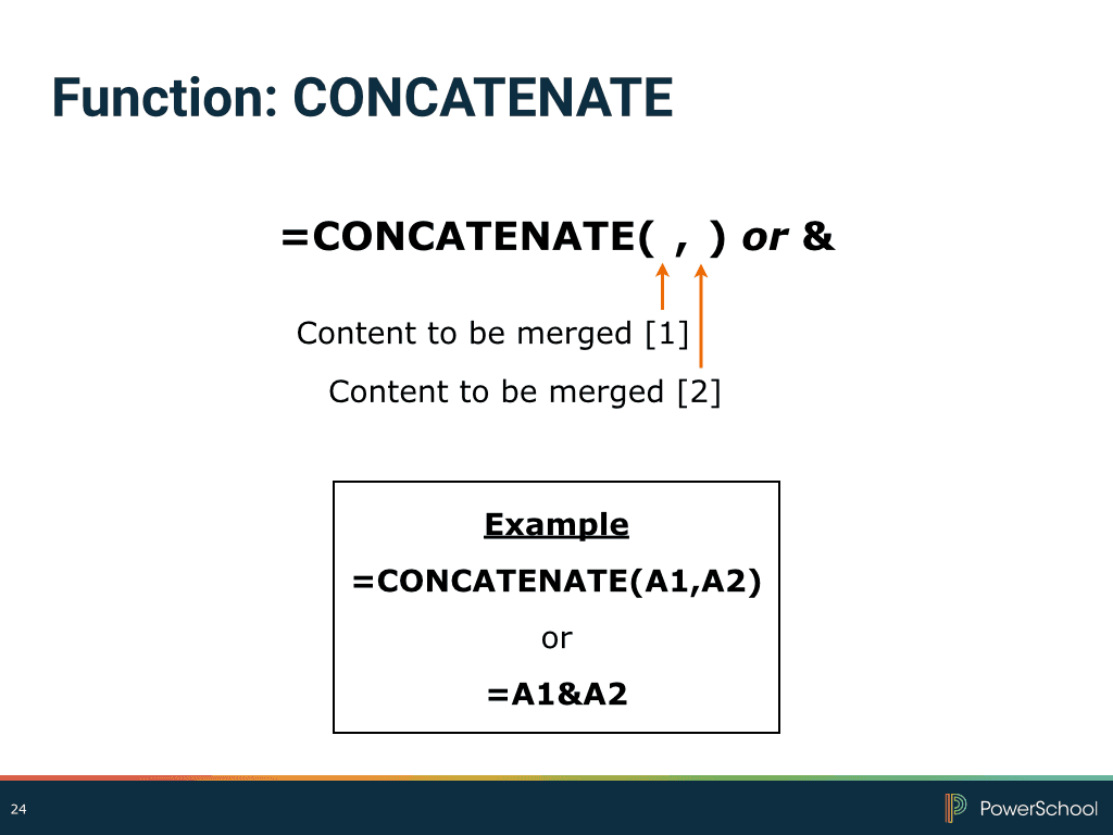
First, explore the CONCATENATE function. The Concatenate function is one of the most common and useful functions in Excel. So much so, in fact, that there’s a shorthand way of writing it: use an ampersand.

Concatenate, or the ampersand, merges the contents of multiple cells together into one. This is not a mathematical operation, so if you use it on cells containing numbers, you’ll get one larger number consisting of the smaller numbers pasted together.

This function can be useful for many tasks, from merging teacher comments or test scores to creating usernames and passwords from users’ personal information.

Interaction 4 – Slides

Review how to use the CONCATENATE function and text in quotes. Click to view slide(s).

Activity 4 – Using Concatenate to Combine Data and Add Text to Create New Data Sets

Use teachers’ first and last names to create teacher email addresses in the format Deborah.Davis@aghs.org.

1. On the Teacher Info worksheet, in the first cell under the Email heading, enter an = sign to start the formula
    
2. Enter the first cell that you want to combine to create the email address:
   =D2
    
3. Enter an ampersand & to concatenate one string with another:
   =D2&
    
4. Since you need a period between the first and last names, enter ”.” after the ampersand:
   =D2&”.”
   The quotation marks tell Excel to consider the text between them as a string on its own rather than using the text as part of a cell reference or other operation.
    
5. Add another ampersand, and then enter your next cell reference, C2:
   =D2&”.”&C2
    
6. Add another ampersand and the email domain information, remembering to put the text in quotes:
   =D2&”.”&C2&”@aghs.org”
    
7. Press Enter
    
8. Autofill the formula down the column by placing your cursor in the bottom-right corner of the cell you entered the formula into so it turns to a black + sign, then clicking and dragging down the column to the last row of data
   Alternatively, you can autofill by double-clicking when the cursor turns into a black plus sign. Excel will then autofill the formula down to the last row of data for you. For this activity, this method will work for Excel 2013 users, but Excel 2016 requires that the column to the left of the one to be autofilled be populated, so it will not work here (but will work for the next activities).

Activity 5 – Using The Left and Lower Functions

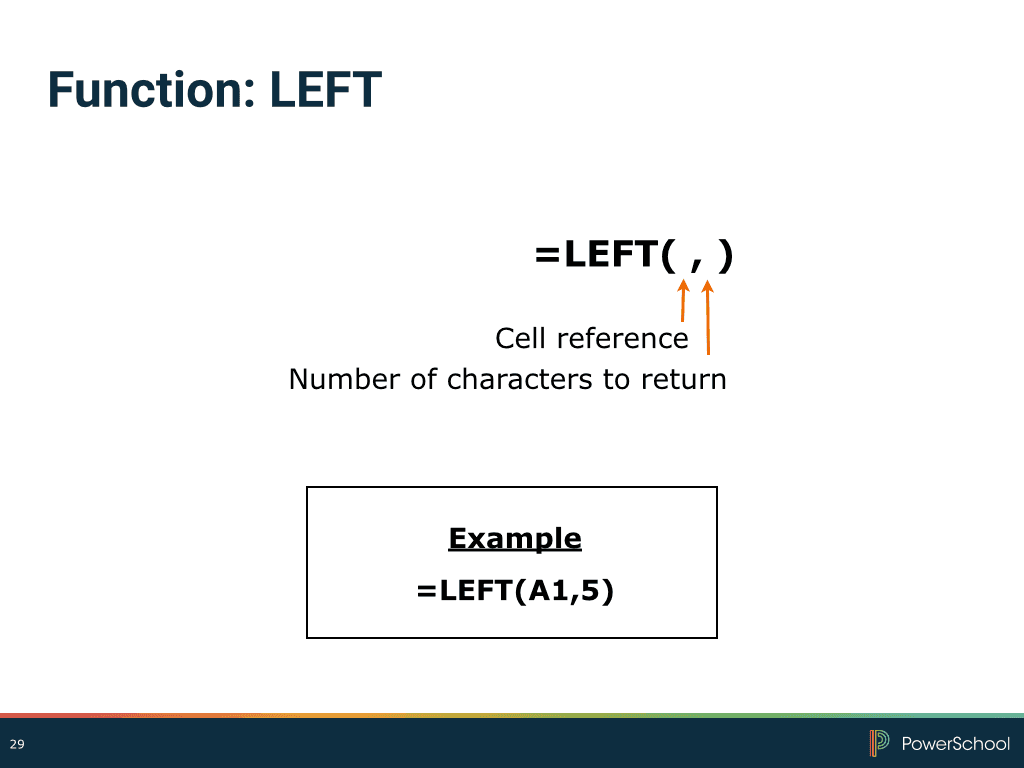
The LEFT function returns a string of characters from a cell, starting from the first, or left-most, character. The cell is determined by the first argument, and the number of characters is determined by the second argument.

The LOWER function changes any capital letters in a string of text to lowercase.

Interaction 5 – Slides

Review how to use the LEFT and LOWER functions. Click to view slide(s).

Use these functions to create usernames for teachers consisting of the first letter of their first names followed by their last names. Use the LEFT function to extract the proper information, and the LOWER function to change any capital letters to lowercase.

1. On the Teacher Info worksheet, in the first cell under the Username heading, begin the LEFT function:
   =LEFT(
    
2. Enter the cell containing the teacher’s first name, D2, as the first argument, followed by a comma:
   =LEFT(D2,
    
3. Enter the number of characters you want to return, 1, as the second argument and end it with ):
   =LEFT(D2,1)
    
4. Insert the teacher’s last name by adding &C2 to the end of the formula:
   =LEFT(D2,1)&C2
    
5. To make all characters lowercase, wrap your formula in the LOWER function:
   =LOWER(LEFT(D2,1)&C2)
    
6. Press Enter, then autofill the formula down the column

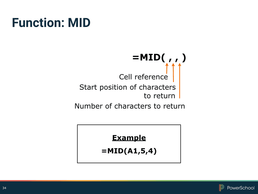
Activity 6 – Using The Mid Function

The MID function returns a certain number of characters, starting from a certain position, from a specified cell. The first argument in the function is the cell you want to pull the characters from. The second argument is the position in the cell that you want to start pulling from. The third argument is the number of characters you want returned.

Interaction 6 – Slides

eview how to use the MID function. Click to view slide(s).

Use the MID function to create passwords for the teachers in your worksheet. The passwords should consist of the first letter of the teacher’s last name followed by the teacher number, minus the leading “10-.”

1. On the Teacher Info worksheet, in the first cell under the Passwords heading, begin your formula with a LEFT function that will return the first letter of the teacher’s last name, followed by an ampersand:
   =LEFT(C2,1)&
    
2. Next, enter the start of a MID function:
   =LEFT(C2,1)&MID(
    
3. Enter the cell containing the teacher number, A2, as the first argument, followed by a comma:
   =LEFT(C2,1)&MID(A2,
    
4. Enter the position within the cell of the start of the string you want to extract, 4, as the second argument, followed by a comma:
   =LEFT(C2,1)&MID(A2,4,
    
5. Enter the number of characters you want to extract, 5, as the third argument, and end it with ):
   =LEFT(C2,1)&MID(A2,4,5)
    
6. Press Enter, then autofill the formula down the column

Activity 7 – Using The Right Function

The RIGHT function is similar to the LEFT function, but it returns a number of characters from the last, or right-most, character.
Use the Right function to extract science scores that are embedded as the last two characters in state exam scores.
Note that since the RIGHT function is a text function, Excel will treat the value that gets returned as text. In a later activity you’ll perform some mathematical operations on these values, so you’ll have to take an extra step to make Excel consider the value as numeric.

1. On the State Exam worksheet, in the first cell under the Science Score heading, begin the RIGHT function:
   =RIGHT(
    
2. Enter the cell containing the state exam score, G2, as the first argument, followed by a comma:
   =RIGHT(G2,
    
3. Enter the number of characters you want to return, 2, as the second argument and end the formula with ):
   =RIGHT(G2,2)
    
4. Press Enter, then autofill the formula down the column
    
5. Use what you’ve learned about the LEFT and MID functions to extract the first two characters into the Math Score column, and the third and fourth characters into the English Score column
   
   Since the RIGHT, LEFT, and MID functions are text functions, complete an extra step to make Excel consider the returned values as numeric. There are two ways to do this:
   
   – Nest your text function in a VALUE function. The VALUE function converts a text string that represents a number to a number.
   
   - Perform a mathematical operation on the result of the function that won’t change the value, such as adding 0, multiplying by 1, or inserting two negative signs in front of the function name (effectively multiplying the value by negative 1 twice)
    
6. Use either method listed above to convert the values in the Math Score, English Score, and Science Score columns to numerical values
   For example, the first cell under the Science Score heading could contain one of the following formulas:
   
   =VALUE(RIGHT(G2,2)) =RIGHT(G2,2)+0 =RIGHT(G2,2)*1 =–RIGHT(G2,2)

Activity 8  – Using The Len Function

The LEN, or LENGTH, function returns the number of characters in a cell. This function is useful if you need to know which cells contain the least or most characters, or which cells contain fewer or more than a certain number of characters.

Interaction 7 – Slides

Review how to use the LEN function. Click to view slide(s).

Your district is now limiting the number of characters allowed for course names to 20. Use the LEN formula to determine which courses will need to have their names shortened.

1. Open the Course Names worksheet
2. In the first cell under the Length of Course Name heading, begin the LEN function:
   =LEN(
3. Enter the cell number for the course name, A2, and end with ):
   =LEN(A2)
4. Press Enter
5. Autofill the formula down the column
6. Sort the data by the “Length of Course Name” column in descending order
   1. Click the box just above the row numbers to highlight all the cells on the worksheet
   2. Click the Data tab in the ribbon
   3. Click Sort
   4. In the menu under Column, select Length of Course Name
   5. In the menu under Order, select Largest to Smallest
   6. Make sure “My list has headers” is selected, and click OK

How many courses have names longer than the 20-character maximum?

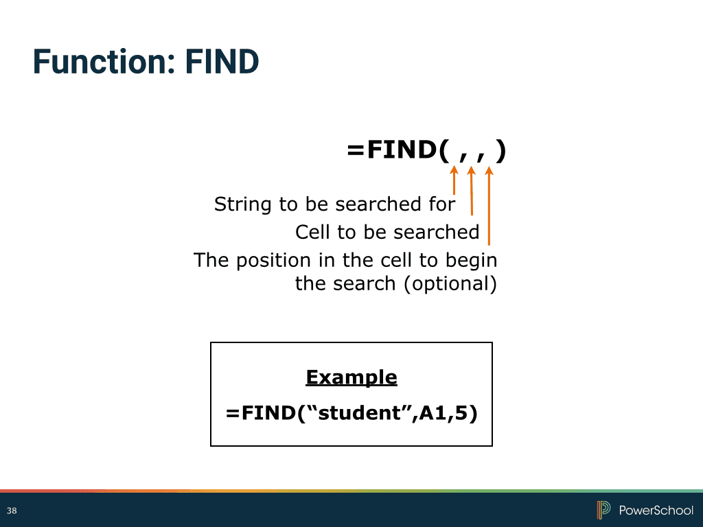
Activity 9 – Using the Find Function

The FIND function returns the starting position of a text string in a cell. The first argument is the string you want to search for. This can be a cell that contains your search term, or you can enter the search term in quotes to define the term in the formula. The second argument is the cell to be searched. The third argument is the position in the cell that you want the search to start. If you leave this argument out, the search will start at the first position in the cell.

The FIND function is case sensitive, so it’s important to ensure that your search term uses capital and lowercase letters in the same way as the text you search.

Interaction 8 – Slides

Review how to use the FIND function. Click to view slide(s).

Since the FIND function returns a position in a cell, it’s commonly used in other formulas.
 

For this activity, imagine you need to extract just the street numbers from students’ addresses. Use the FIND function to get the required information.

1. Switch to the Student Info worksheet
    
2. In the first cell under the Street Number heading, start the formula:
   =FIND(
    
3. Enter your search term in quotes as the first argument; since all the street numbers are followed by a space, enter ” “:
   =FIND(” “
    
4. Now add a comma and enter the cell to be searched, D2, followed by a closed parenthesis:
   =FIND(” “,D2)
    
5. Use your FIND function as the second argument in a LEFT function to return the text in the address column up through the first space:
   =LEFT(D2,FIND(” “,D2))
    
6. To keep the space from being returned as well, add -1 after the FIND function:
   =LEFT(D2,FIND(” “,D2)-1)
   Since the FIND function returns a number, you can use mathematical operations on it and subtract it by 1.
    
7. Press Enter, then autofill the formula down the column

Using Date Functions

The next set of functions and formulas pertain to date data. Like text, elements can be extracted from dates, but unlike text, dates can be altered with mathematical operations.
 

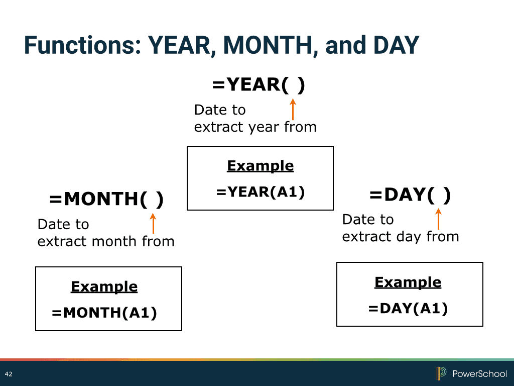
Activity 10 – Using the The Month, Day, and Year Functions

The YEAR, MONTH, and DAY functions all work in a similar way. They return the year, month, or day of a date. In order for them to return valid values, the arguments must point to a date.

Interaction 9 – Slides

Review how to use the MONTH, DAY, and YEAR functions. Click to view slide(s).
Split students’ dates of birth into separate columns using the MONTH, DAY, and YEAR functions.

1. Make sure you’re still on the Student Info worksheet
    
2. In the first cell under the Birth Month heading, enter:
   =MONTH()
    
3. Enter the cell containing the student’s date of birth as the argument, F2:
   =MONTH(F2)
    
4. Press Enter, then autofill the formula down the column
    
5. The DAY function is similar to the MONTH function, so in the first data cell in the Birth Day column, enter:
   =DAY(F2)
    
6. Press Enter, then autofill the formula down the column
    
7. Enter the YEAR function in the Birth Year column:
   =YEAR(F2)
    
8. Press Enter, then autofill the formula down the column

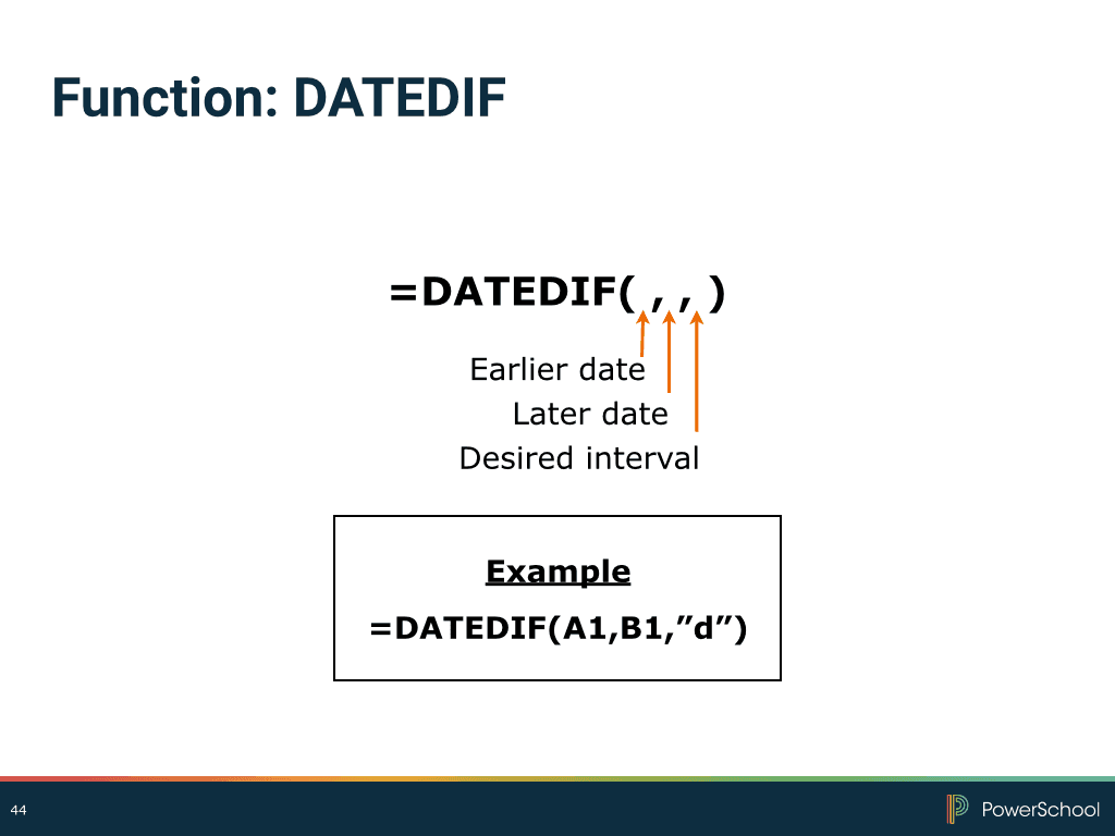
Activity 11 – Using The DATEDIF and TODAY Functions

The DATEDIF formula returns the difference between two dates. The first argument is the earlier date. The second argument is the later date. The interval of time in which the result is shown is determined by the third argument. See the table at the end of this course material for the interval options.

The TODAY function returns today’s date, and doesn’t require an argument between the parentheses.

Interaction 10 – Slides

Review how to use the DATEDIF and TODAY functions. Click to view slide(s).
Use students’ dates of birth, as well as today’s date, to determine their current ages using the DATEDIF and TODAY functions.

1. On the Student Info worksheet, in the first cell under the Current Age heading, enter:
   =DATEDIF(
    
2. The earlier date is the student’s date of birth, so enter F2 as the first argument, followed by a comma:
   =DATEDIF(F2,
    
3. Use today’s date as the second argument by entering the TODAY function, followed by a comma:
   =DATEDIF(F2,TODAY(),
    
4. Since you want the student’s age to appear in years, enter “y” as the third argument, followed by a ):
   =DATEDIF(F2,TODAY(),”y”)
    

For the other intervals available, see the list of functions at the end of this course material.

Press Enter, then autofill the formula down the column

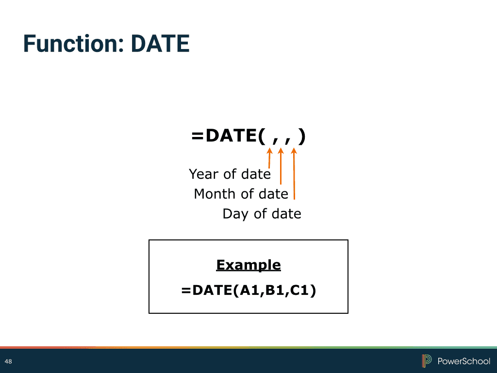
Activity 12 – Using The Date Function

The DATE function returns a date. The year, month, and day of the date returned are determined by the three arguments in the formula. The DATE function is often used along with the YEAR, MONTH, or DAY functions to pull elements from other dates and create new ones.

Interaction 11 – Slides

Review how to use the DATE function. Click to view slide(s).
Determine the date that students will turn 16 and become eligible for Driver’s Education using the Date function.

1. On the Student Info worksheet, in the first cell under the Date Eligible for Driver’s Ed heading, enter:
   =DATE(
    
2. Enter the YEAR, MONTH, and DAY functions as the arguments for the DATE formula, followed by a ):
   =DATE(YEAR(F2),MONTH(F2),DAY(F2))
    
3. Students become eligible for Driver’s Ed when they turn 16, so add 16 to the year in your formula:
   =DATE(YEAR(F2)+16,MONTH(F2),DAY(F2))
    
4. Press Enter, then autofill the formula down the column

Activity 13 – Combining The DATEDIF and DATE Functions

Use the DATEDIF and DATE functions together to determine students’ ages on the first day of school. Assume the first day of school is September 1, 2015.

1. On the Student Info worksheet, in the first cell under the “Age on first day of school” heading, enter:
   =DATEDIF(
    
2. The earlier date is the student’s date of birth, so enter F2 as the first argument, followed by a comma:
   =DATEDIF(F2,
    
3. To use the date of the first day of school as the second argument, enter a DATE function with the first day’s year, month, and day as its arguments, followed by a comma:
   =DATEDIF(F2,DATE(2015,9,1),
    
4. Since you want the student’s age to appear in years, enter ”y” as the third argument of the DATEDIF function, followed by a ):
   =DATEDIF(F2,DATE(2015,9,1),”y”)
    
5. Press Enter, then autofill the formula down the column