Microsoft Excel is a spreadsheet program, and is a powerful tool you can use to store, organize, and manipulate your PowerSchool data. During this course, you will learn:

• Basic Excel concepts and terminology
• How to change the appearance of data
• How to sort and filter data records
• How to use formulas and functions to analyze and calculate data
• How to adjust settings to prepare your file to print

Note: The instructions in this course are written for Excel 2016 for Mac and Excel 2013 for PC. The instructions for other versions may differ slightly from those shown here.

Basic Excel Concepts

Before delving into working with data, take a look at how Excel organizes information on the page, and how its tools are organized.

Open the activity file called Excel_Basics.xls and use it to explore the parts of Excel discussed below.
 

Columns, Rows, and Cells

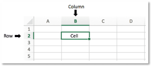
In general, Excel organizes data using a table format made up of columns, rows, and cells. Columns are identified by letters and rows by numbers. A cell is referred to by its column letter and row number. In the image below, the selected cell would be called “cell B2.”

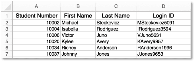
Typically, data records are entered into the rows of Excel, with similar data for each record being organized into columns. The first row frequently contains titles for the columns of data below it; these titles are called “column headings,” and are often formatted differently than the rest of the data in order to differentiate them.

Worksheets and Workbooks

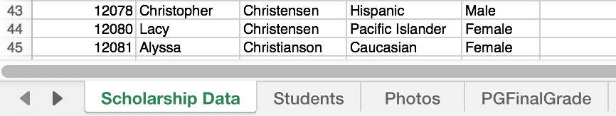
In Excel, each spreadsheet page is called a “worksheet,” and a file containing one or more worksheets is called a “workbook.” By default, worksheets have the name “Sheet1,” “Sheet2,” etc., but it’s a good idea to rename your worksheets to reflect the data they contain.

Toolbars

The top of an Excel worksheet contains several toolbars, and each toolbar contains its own set of tools.

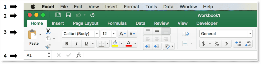
Here are the toolbars for Excel 2016 for Mac:

(If you use a different version of Excel, some of your options may appear in a different order or format.)

1. Menu bar – Access most of Excel’s tools either through these menus or the Ribbon
2. Quick Access toolbar – Includes the File button, which contains commands to open a new, recently used, or saved workbook; the toolbar also has Save, Undo, and Redo buttons
3. Ribbon – Access the majority of the commands that you’ll use
   The Ribbon is grouped into individual tabs. A few examples include:
          
   Home tab – Contains tools for formatting cells
   Formulas tab – Lists the different functions in Excel by type
   Data tab – Contains such commands as Sort and Filter
    
4. Formula bar – Use to view and edit the formula in a selected cell

Here are the toolbars for Excel 2013 for PC:

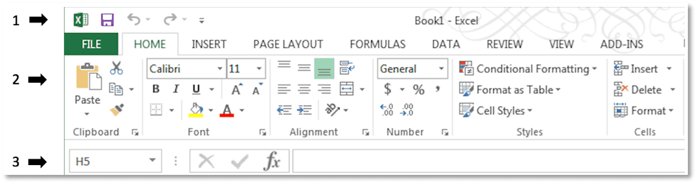
1. Quick Access toolbar – Contains Undo, Redo, and Save buttons
2. Ribbon – Excel 2013 for PC doesn’t include the Menu bar, and instead relies on the Ribbon for nearly all of its functionality
   The Ribbon is grouped into individual tabs. A few examples include:
   
   File tab – Unique to the PC version of Excel; opens a separate window that includes commands to open a new workbook, print a worksheet, and access Excel preferences
   
   Home tab – Contains tools for formatting cells
   
   Formulas tab – Lists the different functions in Excel by type
   
   Data tab – Contains commands such as Sort and Filter
    
3. Formula bar – Use to view and edit the formula in a selected cell

Note: Versions of Excel not shown here may display options in a different order or format, but the functionality is the same.

The Ribbon

The Ribbon is the go-to toolbar for all your data manipulation needs. The Ribbon is made up of multiple tabs, each containing a category of tools, options, and settings for you to apply to your data. Take a look at the table below to review each of the tab names, brief descriptions of each tab, and some of the most frequently used tools that each tab contains.

Tab Name	Description	Frequently Used   Tools
File (Unique to the PC version; in the Mac version, the commands on this tab appear in the Excel and File menus of the Menu bar)	Commands that create or affect Excel files as a whole	Create new workbook  Preferences Print
Home	Formatting tools used to alter the appearance of your data	Text font, size, color, and alignment Cut, copy, and paste Format painter Cell border options
Insert	Options for objects that can be inserted into your worksheet	Pivot Tables Charts Images Comments
Page Layout	Options that affect what the worksheet will look like when it is printed	Margins Print area Rows and columns to repeat on each page
Formulas	Tools and options surrounding the building of formulas	Formula Builder (accessed by clicking Insert Function) AutoSum Named ranges Show formulas
Data	Tools for analyzing and manipulating data on the worksheet	Sort Filter Text to columns Remove duplicates
Review	Tools for checking, protecting, and commenting on data	Spell check New comment Protect sheet / workbok
View	Options regarding how the worksheet appears and acts on the screen	Normal / page layout Zoom Freeze panes

Formatting Your Data

Using Excel’s default formatting is fine, but to create professional-looking worksheets that clearly present your data, you’ll need to apply some custom formatting. In the following activities, explore how to use the Ribbon’s Home tab, as well as the Format Cells window, to change the appearance of your data.

Activity 1 – Using the Ribbon’s Home Tab to Apply Formatting

Use the formatting options in the Ribbon to customize the look of a worksheet.

1. With the Excel_Basics.xls activity file open, select the PowerSchool Export worksheet
   
   Data that is exported from PowerSchool will typically look a lot like this when opened in Excel. The worksheet is functional as it is, but could use some formatting adjustments to make it appear professional and easy to read.

Bolding

Make your column headings stand out by bolding them.

2. Select all the cells in the first row, which contains your column headings, by clicking the row number 1

3. Make the column headings bold by clicking the Bold button in the Ribbon

You may notice that many of the column headings, as well as many of the data values don’t fit in their cells. You’ll adjust the column widths to fit the values in a later activity.
 

Adjusting Font Size

Increase the size of your column headings to make them easier to read.

4. With the cells in the first row still selected, click the arrow next to the Font Size menu in the Ribbon

5. Select 14 from the menu
 

Changing Cell Color

Add some style to the header row by adjusting the background color.

6. Since only the cells containing the column headings should have color added, rather than the entire first row, select only the cells in the first row that contain text; this can be done in one of three ways:

• Click and drag your cursor from cell A1 to cell M1
• Click cell A1, press and hold the Shift key, and then click cell M1
• Click cell A1 and press Command + Shift + the right arrow(Control + Shift + the right arrow on a PC)

7. In the Ribbon, click the arrow next to the Paint Bucket button

8. Select a color from the color options (preferably a light color so the black font will be legible)

Aligning Text

Center the column headings within their cells.

9. With the column headings still selected, click the Center Align button in the Ribbon

10. Click the Save button at the top of the window to save your work
 

Activity 2 –Using the Format Cells Window to Apply Formatting

Another way to apply formatting to your data is to use the Format Cells window. Most of the formatting options that appear in the Format Cells window are also available in the Ribbon, but there are a few differences.

Use the Format Cells window to continue to customize the PowerSchool Export worksheet.

Adding a Cell Border

Make your column headings stand out even more by adding a border around them.

1. With your column headings still selected, right-click any of the selected cells

Alternately, on a Mac, press and hold Control and left-click any of the selected cells.

2. From the menu, select Format Cells

3. In the Format Cells window, select the Border tab

4. In the Line Style area, select one of the solid line options

5. Under Presets, select both Outline and Inside

Notice that under Border, a preview of the borders appears. You can click the lines in the Border area to adjust the borders.
 

6. Click OK

The column headings now have borders surrounding them. You may notice that the headings that don’t fit in their cells don’t have complete borders. When you adjust the column widths in a later activity, the complete borders will appear.

Changing Value Categories

The Semester 1 percentage grades in column J are currently in decimal form. Change the formatting of the cells so that the grades appear as percentages.

7. Select all of the S1 percentage grades in column J, and do not include the column heading; this can be done in one of three ways:

• Click and drag your cursor from cell J2 to cell J267
• Click cell J2, scroll down until the last value in the column is visible, press and hold the Shift key, and click cell J267
• Click cell J2 and press Command + Shift + the down arrow(Control + Shift + the down arrow on a PC)

8. Right-click any of the selected cells

9. From the menu, select Format Cells

10. In the Format Cells window, select the Number tab, and choose Percentage from the Category list

Changing a value’s category doesn’t change the value itself. It just changes how the value appears in the cell.
While you’re here, take note of the other category options.

11. Next to the decimal places number, click the down arrow until you get a value of “0″

Notice that a sample result appears above the decimal places selection, and shows you what your values will  look like after you’re done making your changes.

12. Click OK
      The S1 percentage grades now appear as percentages.
 

Wrapping Text

Many of the students’ names in column D consist of more characters than will fit in the width of the column. Change the cell settings to wrap the text in these cells.

13. Select all of the students’ names in column D by clicking cell D2, and then pressing Command + Shift + the down arrow (Control + Shift + the down arrow on a PC)
 

14. Right-click any of the selected cells
 

15. From the menu, select Format Cells

16. In the Format Cells window, click the Alignment tab

17. Under “Text control,” select Wrap text

18. Click OK

The students’ names now wrap within their cells, and the height of the rows is adjusted to fit the names, when necessary.
 

Activity 3 – Manipulating Rows and Columns

You’ve learned some great techniques for adjusting the formatting of your cells. Now learn how to make changes to the appearance of your worksheet’s rows and columns.

Continue working with the PowerSchool Export worksheet for this activity.

Resizing Columns to Fit Values

Many of your column headings and data values contain more characters than can fit within the width of your columns. Adjust the column widths to fit your data.

1. Resize a single column, column A, in one of three ways:

• Place your cursor between column letters A and B so it becomes a vertical bar with two horizontal arrows, and then click and drag your cursor to the right to make the column as wide as you’d like
• Place your cursor between column letters A and B so it becomes a vertical bar with two horizontal arrows, and then double click; the column resizes automatically to fit the widest value in the column
• Right-click the column letter A, select Column Width from the menu, enter a column width value (such as 1.5), and click OK
   

2. Resize all of your columns at once; first select all your worksheet’s values by clicking and dragging your cursor from column letter A to column letter M, and then complete one of the following three steps:

• Place your cursor between any two of the selected columns so it becomes a vertical bar with two horizontal arrows, and then click and drag your cursor to the right
  
  All the columns will be resized at once.
• Place your cursor between any two of the selected columns so it becomes a vertical bar with two horizontal arrows, and then double click; the columns will be resized automatically to fit the widest value in the columns
• Right-click any of the selected columns’ letter, select Column Width from the menu, enter a column width value (such as 1.5), and click OK

Inserting Columns

The Student Fees worksheet contains the fees that each of your students owes. Add this data as a new column just to the left of what is currently column M.

3. Start by clicking column letter M to highlight the entire column
 

4. Insert a new column just before the highlighted column in one of two ways:

• On the Home tab in the Ribbon, click Insert
• Right-click any of the selected cells, and choose Insert from the menu
• A blank column is inserted.

5. Click the Student Fees worksheet tab towards the bottom of the Excel window
 

6. Select the values in column B, including the column heading
 

7. Copy the values in one of two ways:

• Click Copy in the Home tab of the Ribbon
• Press Command + C (or Control + C on a PC)

8. Click the PowerSchool Export worksheet tab
 

9. Click cell M1
 

10. Paste the copied values in one of two ways:

• Click Paste in the Home tab of the Ribbon
• Press Command + V (or Control + V on a PC)

Notice that the column heading for column M doesn’t include the formatting you built for the other columns. You’ll learn how to copy formatting in a later activity.
 

Inserting Rows

Imagine you have another student’s record to add to your worksheet, and you want to insert it as the third row. Insert a new, blank row for the data to be entered into.

11. Click row number 3 to highlight the entire row
 

12. Insert a row just above the highlighted row in one of two ways:

• On the Home tab in the Ribbon, click Insert
• Right-click any of the selected cells, and choose Insert from the menu
  
  A blank row is inserted.

13. Make up and enter values for each cell to create the student’s record
 

Freezing Panes

Since you have a large number of columns and rows that contain data in your worksheet, freeze the first row and column so they stay visible when you scroll.

14. To freeze just the header row, click the View tab in the Ribbon, and click Freeze Top Row (PC users, click Freeze Panes, and then select Freeze Top Row)

Now when you scroll down the worksheet, the first row remains visible.
Unfreeze the row by clicking Unfreeze Panes (PC users, click Freeze Panes, and then select Unfreeze Panes).
 

15. To freeze just the first column, make sure you have the View tab in the Ribbon selected, and click Freeze First Column (PC users, click Freeze Panes, and then select Freeze First Column)

Now when you scroll the worksheet to the right, the first column remains visible.

Unfreeze the column by clicking Unfreeze Panes (PC users, click Freeze Panes, and then select Unfreeze Panes).

16. To freeze both the first row and the first column, click the cell that is just below the row you want to freeze and to the right of the column you want to freeze (cell B2), and on the View tab of the Ribbon, click Freeze Panes (PC users, click Freeze Panes, and then select Freeze Panes)

Now when you scroll in any direction, both the first row and first column remain visible.

 

Hiding Columns

To make it easier to compare the values in two columns, it can be useful to hide the columns between them. Hiding columns doesn’t delete them; it just removes them from view. Hide columns E through J to make it easy to see student’s names with their associated Semester 1 letter grades.
 

17. Select columns E through J

18.  Hide the columns in one of two ways:

• Click the Home tab in the Ribbon, click Format, and from the Hide & Unhide menu select Hide Columns
• Right-click any of the selected cells, and select Hide from the menu
  
  Now the students’ names appear next to their Semester 1 letter grades.

19. To unhide the columns, select columns D through K, and do either of the following:

• Click Format in the Home tab of the Ribbon, and from the Hide & Unhide menu select Unhide Columns
• Right-click any of the selected cells, and select Unhide from the menu

All the columns are now visible again.
 

Common Tools and Shortcuts

Excel contains many tools that you can use to save time for tasks that could be done manually, but would be tedious. A few of the especially useful tools include:

• Format Painter – Applies any formatting that is used on one cell or set of cells to another cell or set of cells
• Lists – Excel is able to recognize and autofill several types of lists, such as numbers in a pattern, days of the week, and months of the year
• Sorting – Puts your data in order according to your chosen criteria
• Filtering – Hides from view any records that contain values you don’t want to see

Activity 4 – Using the Format Painter

Use the Format Painter to make all of the column headings on the PowerSchool Export worksheet look the same.

1. Select any of the column heading cells that have the custom formatting applied
2. On the Home tab of the Ribbon, click the Format Painter tool (looks like a paint brush)
3. Click cell M1, which contains the unformatted column heading you copied earlier
   
   The custom formatting is applied to column M’s heading.
   You can use the Format Painter to apply formatting to multiple cells as well:

• After clicking the Format Painter button, click and drag your cursor over multiple cells to apply the formatting to all the selected cells.
• Double-click the Format Painter tool to keep it turned on even after you’ve clicked to apply it to a cell or range of cells. Continue selecting cells to apply the formatting. Click the Format Painter button again to turn it off.
   

Activity 5 – Autofilling a List

Use Excel’s ability to recognize a list pattern to create unique login passwords for your students consisting of sequential, four digit numbers.

1. On the PowerSchool Export worksheet, insert a new column between columns D and E, and enter the column heading Password
2. Select cell E2 and enter 1001
3. Select cell E3 and enter 1002
4. Select both cells E2 and E3
5. Place your cursor in the bottom-right corner of the selected cells so it changes to a black + sign, and autofill the list down the column in one of two ways:

• Click and drag down the column until you reach the last cell that needs a value
• Double-click to autofill down the column automatically

Excel recognizes the pattern of the two numbers you entered and uses it to fill the remaining cells in the column.
 

Activity 6 – Sorting and Filtering Data

Use the Sort and Filter tools to gain some insight into your data.
 

Sorting

Make it easier to see which students have the fewest and greatest number of absences by sorting your data.

1. On the PowerSchool Export worksheet, select any of the cells in the S1 Absences column (column O)
2. In the Ribbon, click the Data tab
3. Click the Sort Ascending button
   All the records on the worksheet are sorted in ascending order by their value in the S1 Absences column.
4. Click the Sort Descending button
   Now the records are sorted with the highest number of absences showing first.
    

Filtering

Filter your data to show records for only the female, 12th-grade, Hispanic students.

5. Click any cell that contains a value on the PowerSchool Export worksheet
 Make sure that only one cell is selected.

6. On the Data tab in the Ribbon, click Filter
Notice the column headings all have menu arrows now.

7. Click the filter menu arrow next to the Gender heading

8. In the filter window, clear the Male selection

9. Click anywhere outside the filter window (or click OK on a PC) to make the window disappear

Notice the filter menu arrow next to the Gender heading now has a funnel icon. This indicates that a filter has been applied.
Now look down the Gender column to see that only female students are listed. The data for the male students has not been deleted; it is just hidden from view and will become visible again when the filter is cleared.
 

10. Click the filter menu arrow next to the Grade Level heading and clear all the grade level selections in the filter window except for 12 (then click OK on a PC)

11. Apply a filter to the Ethnicity column so only Hispanic students are shown

The remaining students are your female, 12th-grade, Hispanic students.
 

12. Clear the filter for Ethnicity by clicking the filter menu arrow next to the Ethnicity heading and clicking Clear Filter

13. Clear all of the remaining filters and remove the filter menu arrows by clicking Filter on the Data tab in the Ribbon
 

Formulas and Functions

When a formula is entered into a cell, it performs a calculation or action in the background and displays the result in the cell. The Formula bar, which appears just below the Ribbon, displays the formula that was entered into a selected cell, while the cell itself displays the formula’s result.

There are many uses for formulas in Excel. They can perform mathematical and statistical operations, combine text strings, determine if the value in a cell meets a condition, retrieve values from other cells, and many other actions.

One of the most powerful aspects of formulas is that you can use cell references within them. Using cell references makes the result of your formulas dynamic, so as the values in cells that are referred to in your formulas change, the results of the formula also change. Note that when you use cell references in a formula, the formula considers the actual value that appears in the cell being referred to rather than any formula that may be in the background for that cell.

All formulas start with an = sign. When you enter an = sign as the first character in a cell, Excel will always treat it as a formula and attempt to return a value.

Activity 7 – Using a Formula to Sum Values

Use a formula to add up the fees that are owed by 10th-grade students.
 

1. First, filter your data to show only the 10th-grade students
    
2. Enter your formula in the cell just below the list of student fees; click cell N269
    
3. Enter an = sign to start the formula, followed by a mathematical equation that adds up the non-zero fee values:
   =25+7+7+5+23+26+30
    
4. Press Enter
   Excel evaluates the formula and returns a sum of the values.
    
5. Click cell N269 again, and look at the formula in the Formula bar
   The Formula bar displays the formula that is resulting in the value shown in the selected cell.
    
6. Now enter a formula that uses cell references rather than static values; click cell N270
    
7. Enter an = sign to start the formula, followed by a mathematical equation that uses the cell references of the non-zero fee values
   
   To enter a cell reference into your formula, either type it or click the cell itself. The final formula should be:
   
   =N78+N133+N134+N135+N201+N202+N203
    
8. Press Enter
   
   You get the same result as the previous formula, but Excel assumes you want to use the same formatting as the cells you referenced and adds a $ sign.
    
9. Now imagine that student Kris Hopkins pays her fee; click cell N133and change the value to 0
   
   Did either of your formula values change? Why?
    
10. Clear all the worksheet’s filters by clicking Filter on the Data tab of the Ribbon
     

Activity 8 – Using a Formula to Find Values that Meet a Condition

Use a formula to find students whose fees meet certain conditions.

Start by seeing which students owe more than $25.

1. First, give column P the heading Fee Info, and use the Format Painter to give it the same formatting as the other headings
    
2. Click cell P2
    
3. Enter an = sign to start the formula, followed by the cell reference of the student fee for the first student: =N2
    
4. Next, enter a > sign, followed by the value in question, 25:
   
   =N2>25
    
5. Press Enter
   The formula returns “FALSE” since the student’s fee, $0, is less than 25.
    
6. Autofill the formula down the column by clicking cell P2 again, placing your cursor in the bottom-right corner of the selected cell so it becomes a black + sign, and double-clicking
   Look over the results of the autofilled values and verify that students who owe more than $25 in fees have “TRUE” in column P.
   Next, see which students owe exactly $25 in fees
    
7. Click cell P2
    
8. Now click in the formula bar and change the > sign in your formula to an = sign:
   
   =N2=25
   
   This formula asks the question, “Is the value in cell N2 equal to 25?”
    
9. Press Enter and autofill the formula down the column
   
   Now only the students who owe exactly $25 have “TRUE” in column P.
   Now see which students owe less than or equal to $25.
    
10. Click cell P2
     
11. Click in the formula bar and add a < sign just before the = sign:
    
    =N2<=25 This formula asks the question, “Is the value in cell N2 less than or equal to 25?”
     
12. Press Enter and autofill the formula down the column
    
    Now only the students who owe $25 or less have “TRUE” in column P.
     

Using Functions in Formulas

A function in Excel is a built-in, predefined operation that contains variable elements, and is used as part of a formula. There are over 350 functions in the latest version of Excel, but knowing how to use even a few of them will go a long way in assisting you to manage and manipulate your data.

Nearly all Excel functions contain one or more variable “arguments.” The arguments are different for each function. Arguments are the parts of a function that define what data should be considered, what action the function should take, how the result should be presented, etc.

To enter a function in a formula, enter the function’s name, followed by an open parenthesis, the arguments separated by commas (if there’s more than one), and then a close parenthesis. And since functions are used as parts of a formula, don’t forget to start your formula with an = sign. For example, here’s a formula that uses a SUM function to add up the values in three cells:

=SUM(A1,C1,E1)

See the interaction on parts of a function for a clearly labeled image showing the components of a function.
 

Activity 9 – Using the SUM Function

The SUM function adds up the values of each of its arguments. The arguments can be static numbers that you enter, singe cell references, or ranges of cells.

Use the SUM function to add up the fees owed by all your students.

1. Enter your new formula under the formulas you built in the previous exercises; click cell N271
    
2. Start your formula by entering an = sign, the formula name, and an open parenthesis:
   
   =SUM(
    
3. For the argument, enter the range of cells that contain the student fees, N2 through N268, followed by a close parenthesis:
   
   =SUM(N2:N268)
   
   Using a colon between cell references tells Excel to consider all of the cells between, and including, the cells referenced.
    
4. Press Enter
   
   The resulting sum now appears in the cell in which you entered the formula.

Activity 10 – Using the COUNTA Function

The COUNTA function tallies the number of non-blank cells in a range.

Use the COUNTA function to determine how many records in your data are missing Social Security numbers.

1. Enter your formula in the first non-header row of column Q; click cell Q2
2. Start your formula with an = sign, the function name, and an open parenthesis:
   
   =COUNTA(
    
3. For the function’s argument, enter the cell range that contains the student Social Security numbers, F2 through F268, followed by a close parenthesis:
   
   =COUNTA(F2:F268)
    
4. Press Enter
   
   The resulting value is the number of students who have SSNs in their records, but you want the number of students who do not. To get the desired number, subtract the result of the formula from the total number of students.
    
5. Select cell Q2 again, and click in the formula bar
    
6. Modify your formula so the result of the COUNTA function is subtracted from the total number of student records, which is 267:
   
   =267-COUNTA(F2:F268)
    
7. Press Enter
   
   The result is the number of students who do not have SSNs entered into their records.
   Follow-up questions:

• Why did you use 267 as the total number of students when there are 268 rows of data?
   
• What tool (that has been already been covered in this course) could you use to limit the visible records to those that are missing SSNs?
   

Bonus Activity 1 – Using the Formula Builder

The Formula Builder is a handy tool that makes building formulas easy. Instead of needing to remember the requirements for the arguments of functions, the Formula Builder breaks functions out into their separate parts, and describes what needs to be entered for each part.

Use the Formula Builder to create a formula that returns the average number of Semester 1 absences for your students.

1. Click cell Q3
    
2. In the Ribbon, click the Formulas tab
    
3. Click Insert Function
    
4. In the Formula Builder window (Insert Function window on a PC), select AVERAGE from the list of functions
   Notice the description that appears towards the bottom of the Formula Builder window. This can be very helpful in determining if the selected function is what you really need.
    
5. In the Formula Builder/Insert Function window, click Insert Function(or OK on a PC)
    
6. In the “Number1″ text field, enter the range of cells that contains the Semester 1 absences, but this time omit the row numbers; type O:O
   
   By omitting the row numbers, you are telling Excel to consider all of the values in column O. (Excel will ignore any non-numerical values, such as the column heading.)
   
   Notice that a preview of the formula’s result appears in the Formula Builder window.
    
7. Click Done (OK on a PC)
   The result in cell Q3 is the average number of Semester 1 absences.
    
8. Close the Formula Builder window (not necessary on a PC)

Working with Worksheets

You’ve learned how to format and manipulate the data contained in your worksheets. Now take a look at some of the ways you can work with your worksheets as a whole.

To create a duplicate of a worksheet, rather than opening a new, blank sheet and recreating the original sheet manually, copy it using the “Move or Copy Sheet” command.

Add a new, empty sheet into a workbook using the Insert Sheet command. The new sheet will be named “Sheet” followed by a number. Rename the sheet to differentiate it, then move it to a new position in the workbook by dragging and dropping it along the row of sheet names at the bottom of the workbook. Delete a worksheet to remove it from the workbook.

Prepare to print a worksheet by defining the rows and columns you want to appear on the page. Before you print, it’s best to view a preview of what the worksheet will look like and then adjust the print area accordingly. Change the following settings to prepare your document for printing:

• Print area – Select the rows and columns to print
• Page orientation – Choose portrait or landscape
• Header and footer – Define the text that will be displayed at the top and bottom of the page
• Rows to repeat – Define the rows, typically the column headings, that will appear at the top of each page
• Columns to repeat – Define the columns, typically row titles if you have them, that will appear as the first column of each page
• Row and column headings – Choose whether or not to include the row and column headings

Activity 12 – Adding and Removing Worksheets

Create a copy of the PowerSchool Export worksheet so you can modify some of its data in a new sheet while retaining the same columns and formatting of the original. Rename the copy to distinguish it from the original sheet and move it to the end of the set of worksheet tabs. Then create a new, blank worksheet. Finally, delete the new worksheet to remove it from the workbook.

Copy

1. On the PowerSchool Export worksheet, open the window where you’ll create a copy in one of two ways:

• On the Home tab of the Ribbon, open the Format menu and select Move or Copy Sheet
• Right-click the worksheet name towards the bottom of the Excel window and select Move or Copy

2. In the “Move or Copy” window, select Student Fees from the list under “Before sheet”

3.  Check Create a copy

4. Click OK

The copied sheet opens and appears in the worksheet tabs between the original PowerSchool Export worksheet and the Student Fees worksheet. It has the same name as the original, followed by a number in parenthesis.
 

Rename

5. Rename the new worksheet to Student Data in one of two ways:

• On the Home tab of the Ribbon, open the Format menu, select Rename Sheet, and with the worksheet name highlighted, type the new name
• Double-click the worksheet name, and with the worksheet name highlighted, type the new name
   

6. Press Enter
 

Move

7. To move your new worksheet, drag and drop the Student Data tab across the set of worksheet tab names until a small triangle appears after the Student Fees worksheet

Create

8. Create a new, blank worksheet in one of two ways:

• On the Home tab of the Ribbon, click the arrow next to the Insert button and select Insert Sheet from the menu
• Click the + sign that is next to the right-most worksheet tab
   

Delete

9. Delete your new, blank worksheet in one of two ways:

• On the Home tab of the Ribbon, click the arrow next to the Delete button and select Delete Sheet from the menu
• Right-click the worksheet name and select Delete from the menu

Activity 13 – Printing a Worksheet

Before you print a worksheet, make sure you’re printing the data you want, without including any unnecessary cells. First, view a print preview, and then limit the print area by selecting the particular rows and columns you want to appear on the printed page. Then decide if the information is best displayed vertically or horizontally. Finally, use the Page Setup options to define how headers, footers, and row and column headings will appear.

1. Click the Student Data worksheet tab

2. To see what the entire sheet will look like if you were to print it now, do the following:

• On a Mac, click File in the Menu bar and select Print
• On a PC, click the File tab in the Ribbon and select Print

The Print window shows a small scale preview of the worksheet as it will appear on the printed page. Use the scroll buttons to see what all of the pages of the document will look like. Use this method to check what the printout will look like as you define the print options. Click Cancel (or the left-facing arrow on a PC) to close the Print window and return to the workbook.

3. To print only the first 7 columns for the first 35 students, click cell A1and drag the selection area to cell G36

4. Click the Page Layout tab in the Ribbon

5. Click Print Area and select Set Print Area from the menu

6. To flip the page layout so that the sheet prints horizontally, on the Page Layout tab, click Orientation and select Landscape

7. To enter a header and a footer that will appear on each page of the printed document, on the Page Layout tab, click Page Setup (PC users, click the small arrow under Print Titles)

8. In the Page Setup window, click the Header/Footer tab

9. From the Header menu, select Student Data to print the title of the worksheet on the top of each page

10. From the Footer menu, select Page 1 of ? to print the page number and total number of pages at the bottom of each page

11. Click the Sheet tab

12. In the “Rows to repeat at top” field, click the table icon

13. Click cell A1 to include the row titles

14. Click the table icon again to return to the Page Setup window

15. Click OK

Check the preview of the document again by clicking File and selecting Print

If you’re happy with the look and layout of your document, it is ready to print.
 

Key Points

• Excel data is organized in cells, rows, columns, and worksheets; a cell is referred to by its column letter and row number (ex. A1)
• The Ribbon contains most of the tools that are used to format and manipulate Excel data
• The Ribbon’s Home tab, and the Format Cells window, contains options for formatting the presentation of your data
• Use the Format Painter to apply the formatting of one cell to other cells
• Use the Sort and Filter tools to view the data values that meet your chosen criteria
• Formulas work in the “background” of a cell, determine the value that appears in the cell, and are typically made up of one or more functions
• Functions are built-in operations with variable elements that dictate a result
• The Ribbon’s Page Layout tab contains options that determine how a worksheet appears when it is printed